In this post, I want to share examples of how watsonx can enhance the event processing flows you create using IBM Event Processing.
I’ll start by describing how Event Processing and watsonx complement each other.
Then I’ll share a couple of simple examples of what this looks like in action.
Finally, I’ll walkthrough how I built the example flows to show you how you can try doing something like this for yourself, and share tips for how to create flows like this.
Enhancing Event Processing with watsonx
I’ve written before about how Event Processing is a low-code tool for creating event processing flows. Based on Apache Flink, Event Processing makes it easy to process streams of events in a stateful way.
Windows let you aggregate – processing events in the context of other events that have happened before or after, and joins let you correlate – processing events in the context of other streams of events.
Generative AI such as watsonx can be used to take your event processing flows a step further. Once you’ve used Flink to aggregate and correlate multiple raw streams of events, you can use watsonx to summarise and explain the insights you find.

In this post, I’ll share two very simple examples to show how easy it is to get started with this.
I’m focusing on summarization in these examples, but that’s just one way that you can use machine learning models with your event processing projects.
Other examples include:
- clustering – identify groups of related events
- question answering – orchestrate responding to questions
- classification – recognise and categorise events
- extraction – identify key information within events
- and many more
The principle for such projects are similar to what I’ll show below: use the core capabilities of Event Processing to transform, correlate and aggregate multiple raw streams of events, and enhance this using machine learning to intelligently recognise and respond to the output.
Example projects
Summarizing stock market activity
Given a stream of stock market activity, generate an easy-to-understand summary of what has happened every hour.
Input: A Kafka topic with an event every minute detailing stock trade activity over the last minute.
{
    "volume": 111052,
    "open": 168.98,
    "high": 169.11,
    "low": 168.96,
    "close": 169.07,
    "datetime": "2024-05-17 15:59:00",
    "stock": "IBM"
}

{
    "volume": 32374,
    "open": 168.964,
    "high": 168.99,
    "low": 168.95,
    "close": 168.975,
    "datetime": "2024-05-17 15:58:00",
    "stock": "IBM"
}

{
    "volume" : 23239,
    "open" : 168.97,
    "high" : 168.99,
    "low" : 168.93,
    "close" : 168.96,
    "datetime" : "2024-05-17 15:57:00",
    "stock" : "IBM"
}

{
    "volume": 23358,
    "open": 168.89,
    "high": 169,
    "low": 168.88,
    "close": 168.97,
    "datetime": "2024-05-17 15:56:00",
    "stock": "IBM"
}

{
    "volume": 22083,
    "open": 168.9,
    "high": 168.94,
    "low": 168.87,
    "close": 168.87,
    "datetime": "2024-05-17 15:55:00",
    "stock": "IBM"
}

{
    "volume": 23331,
    "open": 168.93,
    "high": 168.98,
    "low": 168.89,
    "close": 168.91,
    "datetime": "2024-05-17 15:54:00",
    "stock": "IBM"
}

  ...


{
    "volume": 3998,
    "open": 168.46,
    "high": 168.46,
    "low": 168.4,
    "close": 168.46,
    "datetime": "2024-05-17 15:01:00",
    "stock": "IBM"
}

{
    "volume": 2617,
    "open": 168.49,
    "high": 168.49,
    "low": 168.44,
    "close": 168.46,
    "datetime": "2024-05-17 15:00:00",
    "stock": "IBM"
}
Use Event Processing to… aggregate the stock trade activity in hourly windows, generating statistical summaries of the activity in this time.
{
    "total volume" : 523637,
    "mean price" : 168.70,
    "low price" : 168.40,
    "high price" : 169.11,
    "opening price" : 168.49,
    "closing price" : 169.07,
    "price standard deviation (population)" : 0.145,
    "price standard deviation (sample)" : 0.146,
    "price variance (population)" : 0.021,
    "price variance (sample)" : 0.021,
    "start" : "2024-05-17 15:00:00",
    "end" : "2024-05-17 16:00:00",
    "stock" : "IBM"
}
Use watsonx to… summarise the numerical aggregate values in a simple English explanation.
The stock’s price fluctuated throughout the hour, starting at 168.49 and reaching a peak of 169.11 before closing at 169.07. This shows that the stock experienced both buying and selling pressure throughout the hour.
The mean price of the stock during the hour was 168.70, which suggests that the overall trend was slightly upward. However, the stock’s price did drop below the mean during the hour, reaching a low of 168.40.
The population variance and sample variance are measures of how spread out the prices are from the mean. In this case, the population variance was 0.021 and the sample variance was also 0.021, indicating that the prices were relatively close to the mean.
The population standard deviation and sample standard deviation give us a sense of the typical distance between the prices and the mean. The population standard deviation was 0.145, while the sample standard deviation was 0.146. This means that the prices were, on average, about 0.146 units away from the mean.
In summary, this data shows that there was a high volume of trading for a single tech stock over a one-hour period, with the stock’s price fluctuating around the mean. The prices were relatively close to the mean, with only a small amount of variation from it.
Output: A Kafka topic with an event every hour containing an easy-to-understand summary of the activity in the last hour.
Demo: Here is an example of a flow like this in action:
youtu.be/XU-WSLeNIwY
Summarizing weather sensor measurements
Given a stream of measurements from sensors in a weather station, generate a weather report every hour.
Input: A Kafka topic with an event every two minutes, that contain measurements from a weather station.
{
    "datetime": "2024-05-26 08:59:33",
    "coord": { "lon": -1.3989, "lat": 51.0267 },
    "base": "stations",
    "main": {
        "temp": 14.15,
        "temp_min": 12.99,
        "temp_max": 15.45,
        "pressure": 1009,
        "humidity": 89
    },
    "visibility": 10000,
    "wind": { "speed": 4.63, "deg": 200 },
    "clouds": { "all": 75 },
    "sys": {
        "type": 2,
        "id": 2005068,
        "country": "GB"
    },
    "timezone": 3600,
    "id": 2652491,
    "name": "Compton",
    "cod": 200
}

{
    "datetime": "2024-05-26 08:57:33",
    "coord": { "lon": -1.3989, "lat": 51.0267 },
    "base": "stations",
    "main": {
        "temp": 14.15,
        "temp_min": 12.99,
        "temp_max": 15.45,
        "pressure": 1009,
        "humidity": 89
    },
    "visibility": 10000,
    "wind": { "speed": 4.63, "deg": 200 },
    "clouds": { "all": 75 },
    "sys": {
        "type": 2,
        "id": 2005068,
        "country": "GB"
    },
    "timezone": 3600,
    "id": 2652491,
    "name": "Compton",
    "cod": 200
}

{
    "datetime": "2024-05-26 08:55:33",
    "coord": { "lon": -1.3989, "lat": 51.0267 },
    "base": "stations",
    "main": {
        "temp": 14.17,
        "temp_min": 12.99,
        "temp_max": 16,
        "pressure": 1009,
        "humidity": 90
    },
    "visibility": 10000,
    "wind": { "speed": 4.63, "deg": 200 },
    "clouds": { "all": 75 },
    "sys": {
        "type": 2,
        "id": 2005068,
        "country": "GB"
    },
    "timezone": 3600,
    "id": 2652491,
    "name": "Compton",
    "cod": 200
}

{
    "datetime": "2024-05-26 08:53:33",
    "coord": { "lon": -1.3989, "lat": 51.0267 },
    "base": "stations",
    "main": {
        "temp": 14.18,
        "temp_min": 12.99,
        "temp_max": 15.45,
        "pressure": 1009,
        "humidity": 93
    },
    "visibility": 10000,
    "wind": { "speed": 4.12, "deg": 200 },
    "clouds": { "all": 75 },
    "sys": {
        "type": 2,
        "id": 2005068,
        "country": "GB"
    },
    "timezone": 3600,
    "id": 2652491,
    "name": "Compton",
    "cod": 200
}

{
    "datetime": "2024-05-26 08:51:33",
    "coord": { "lon": -1.3989, "lat": 51.0267 },
    "base": "stations",
    "main": {
        "temp": 14.17,
        "temp_min": 12.99,
        "temp_max": 16,
        "pressure": 1009,
        "humidity": 90
    },
    "visibility": 10000,
    "wind": { "speed": 4.63, "deg": 200 },
    "clouds": { "all": 75 },
    "sys": {
        "type": 2,
        "id": 2005068,
        "country": "GB"
    },
    "timezone": 3600,
    "id": 2652491,
    "name": "Compton",
    "cod": 200
}

...
Use Event Processing to… aggregate the weather measurements in hourly windows, generating statistical summaries of the measurements taken in this time.
{
    "temperature min": 12.99,
    "temperature max": 17.02,
    "temperature average": 14.88,
    "temperature standard deviation (population)": 0.451,
    "pressure min": 1009,
    "pressure max": 1009,
    "pressure average": 1009,
    "pressure standard deviation (population)": 0,
    "humidity min": 84,
    "humidity max": 90,
    "humidity average": 87,
    "humidity standard deviation (population)": 1,
    "wind speed min": 4.12,
    "wind speed max": 4.63,
    "wind speed average": 4.39,
    "wind speed standard deviation (population)": 0.254,
    "cloudiness min": 75,
    "cloudiness max": 75,
    "cloudiness average": 75,
    "cloudiness standard deviation (population)": 0,
    "start": "2024-05-26 08:00:00",
    "end": "2024-05-26 09:00:00"
}
Use watsonx to… summarise the numerical aggregate values in a simple English explanation.
The pressure remained relatively constant at 1009 millibars, with no significant changes throughout the hour. This consistent pressure indicates stable weather conditions, which would make it feel comfortable for outdoor activities.
Humidity levels varied between 84% and 90%, with an average humidity of 87%. High humidity can make the air feel sticky and uncomfortable, so these readings suggest that it might have been muggy outside during this time.
Wind speed ranged from 4.1 m/s to 4.6 m/s, with an average wind speed of 4.4 m/s. Moderate wind speeds like these can make it feel cooler, as they help to dissipate some heat from the body.
Lastly, the cloud cover remained constant at 75% throughout the hour. While the cloud cover didn’t change, the sun did start to peek through around 9:00 AM, signaling the beginning of a brighter day.
Overall, the weather in Compton, GB on May 26, 2024, was marked by a mix of temperatures, humidity, and cloud cover, with moderate wind speeds making it feel slightly cooler.
Output: A Kafka topic with an event every hour containing an easy-to-understand summary of the weather in the last hour.
Demo: Here is an example of a flow like this in action:
youtu.be/q9LBZiauf0Y
Building these demos
I’m not claiming that these flows are complete and perfect applications. The prompts I used for the watsonx text generation are my quick first attempts. They would absolutely benefit from being more time to experiment in refining them.
Instead, what I want to do with these demos is to illustrate how easy it is to get started, and encourage you to think about how AI APIs such as watsonx could enhance the insights that you could derive from the streams of events that are available in your business.
Stock activity demo
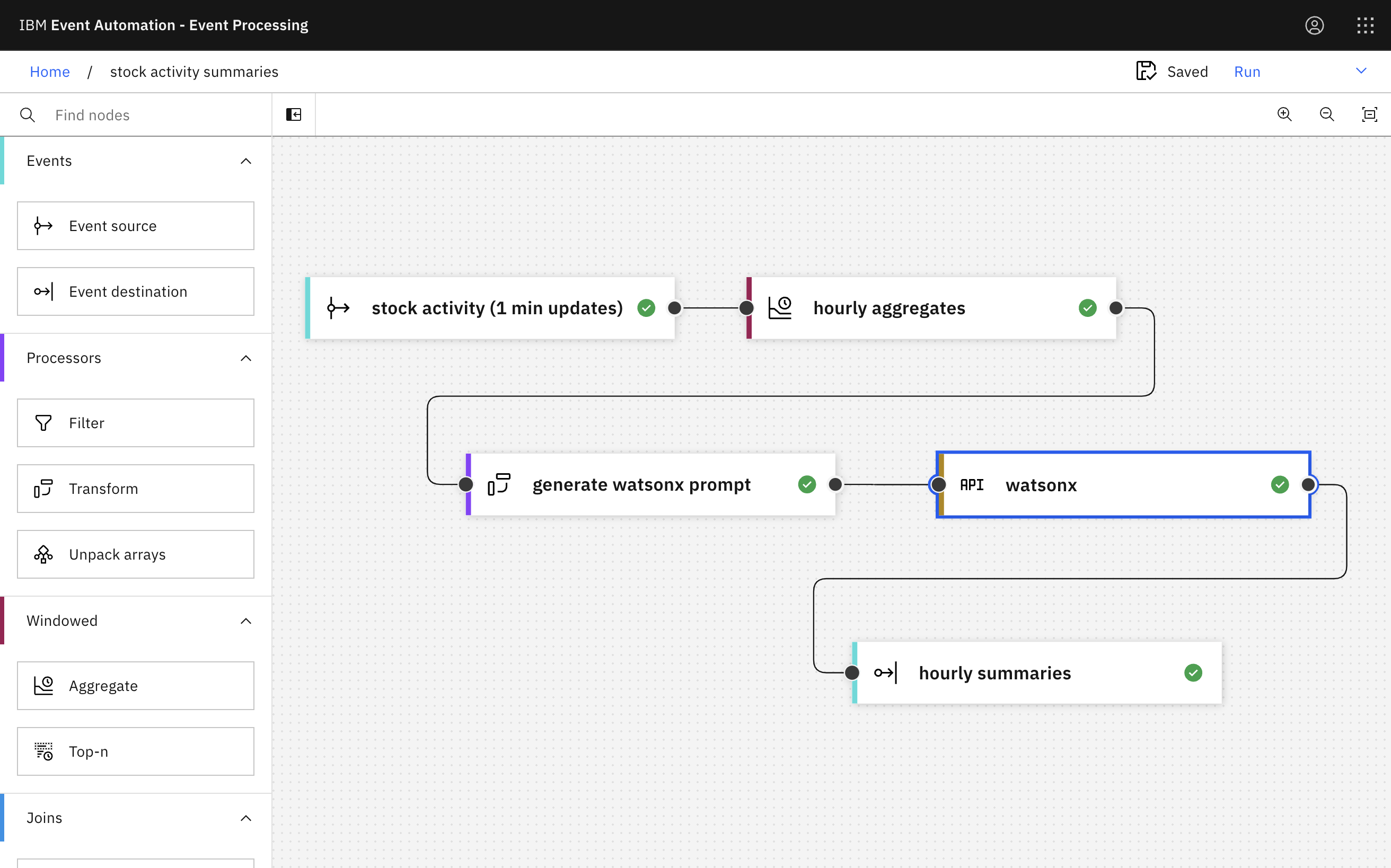
The overall flow looks like this:
I created it like this:
Source of events

The source of events is a Kafka Connect source connector. To see how I set this up, you can see:
- Kafka topic definitions
- Kafka Connect cluster definition
- Source Connector definition
note that it needs a free API key for the Alpha Vantage Stock API which should be added here
The event source node in Event Processing can be configured like this:

Bringing this topic into Event Processing looks like this:

Aggregating
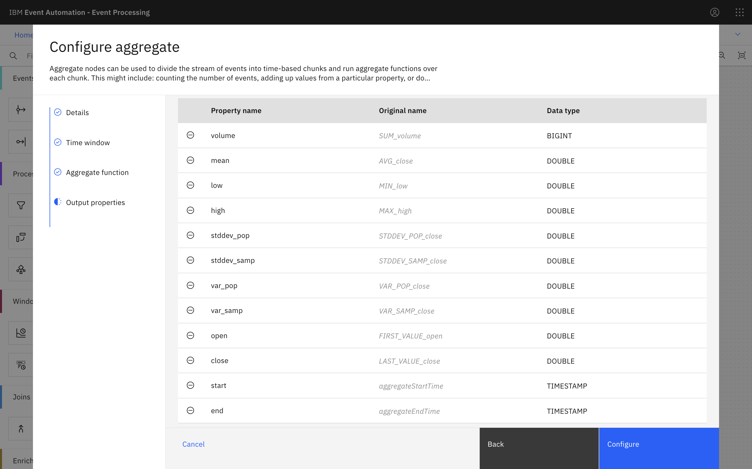
The aggregate node in Event Processing makes it easy to calculate hourly summaries of the stock activity.

There are lots of aggregate functions available to choose from. I picked a selection including SUM, AVG, MIN, MAX, and STDDEV_POP.


Giving the results friendly names makes it easier to use them in processing.
Running this looks like this:

watsonx
The first step is to generate a summarization prompt to use for the model. This can be done using the transform node in Event Processing.

The template I wrote for the prompt is:
CONCAT(
    'These figures describe trading for a single tech stock ',
        'for a 1 hour period between ',
        DATE_FORMAT(`start`, 'yyyy.MM.dd HH:mm:ss'),
            ' and ',
        DATE_FORMAT(`end`, 'yyyy.MM.dd HH:mm:ss'),
    '.\n\n',
    'The number of stocks sold was ',
        CAST(`volume` AS STRING),
    '\n',
    'Trading started at the start of the hour at ',
        CAST(`open` AS STRING),
    ' and finished the hour at ',
        CAST(`close` AS STRING),
    '\n',
    'The highest price during the hour was ',
        CAST(ROUND(`high`, 2) AS STRING),
    '\n',
    'The lowest price was during the hour was ',
        CAST(ROUND(`low`, 2) AS STRING),
    '\n',
    'The average (mean) price was ',
        CAST(ROUND(`mean`, 2) AS STRING),
    '\n',
    'The population variance was ',
        CAST(ROUND(`var_pop`, 3) AS STRING),
    '\n',
    'The sample variance was ',
        CAST(ROUND(`var_samp`, 3) AS STRING),
    '\n',
    'The population standard deviation was ',
        CAST(ROUND(`stddev_pop`, 3) AS STRING),
    '\n',
    'The sample standard deviation was ',
        CAST(ROUND(`stddev_samp`, 3) AS STRING),
    '\n\n',
    'What can we tell about the trading from this data? ',
    'Generate an explanation suitable for someone who is ',
        'not familiar with financial or statistical jargon.'
)
As I said above, I didn’t spend any time refining this. If you would like to improve on this, you can use my example of the sort of prompt this creates to experiment with your favourite large language model. (If you come up with a new prompt that results in a more interesting summary, please let me know!)
The transform node can also remove all the properties that aren’t needed any further in the flow.

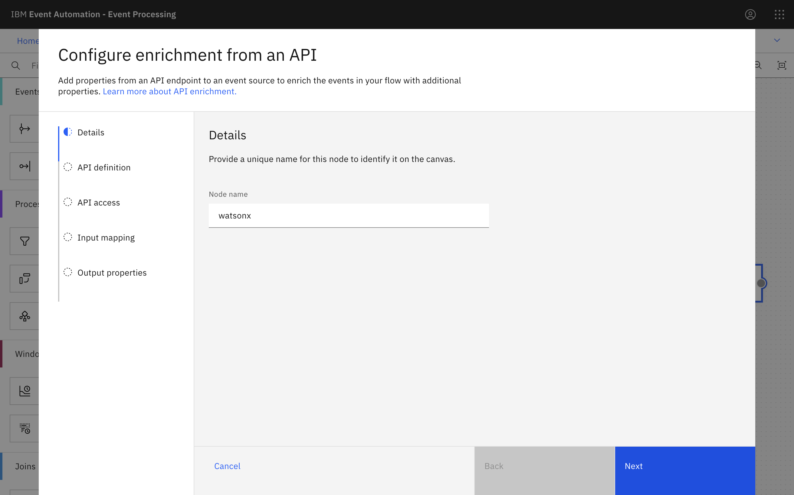
The API Enrichment node in Event Processing lets you enrich the content of events with data retrieved from external REST APIs. It’s useful when you want to process events in the context of reference data from a system of record.
For these demos, I’m using it to invoke a watsonx API.

I prepared a simplified version of the API – simplified both in terms of the auth requirements and the shape of the request and response payloads. Being able to customise the API is one of the benefits of using an AI Gateway. For this demo, I used a simple App Connect flow to play the role of an AI Gateway.
I selected granite-13b-chat but other models are available. For a real project, you would want to experiment with a range of models to identify the best fit for your project.

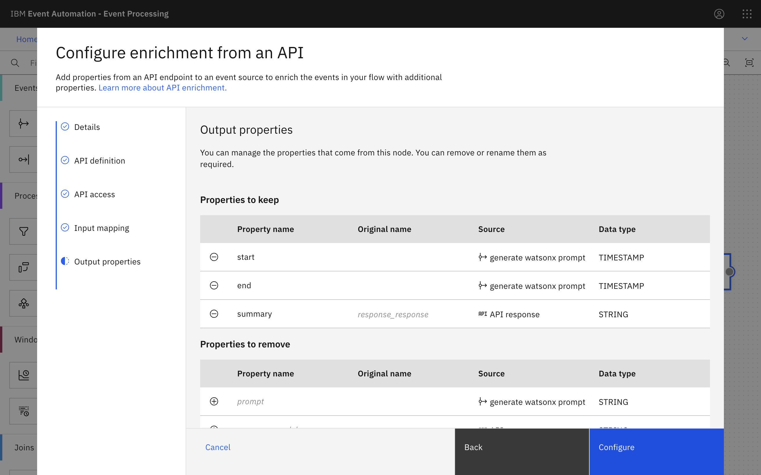
The API Enrichment node can also rename properties and remove properties that aren’t needed, to specify the final output of the flow.

Destination for results
The final step is to sink the output to a new topic.

You can use the output topic as a starting point to trigger notifications, or use a change data connector to sink the generated updates to a database which drives a web or mobile app.

Weather measurements demo
The overall flow looks like this:

I created it like this:
Source of events

The source of events is a Kafka Connect source connector. To see the setup for this, see the:
- Kafka topic definitions
- Kafka Connect cluster definition
- Source Connector definition
note that it needs a free API key for the OpenWeather One Call API which should be added here
The event source node in Event Processing can be configured like this:

The OpenWeather connector includes more data than we need for this demo. I could have used transformations in Kafka Connect to redact the data I don’t need before it reaches the Kafka topic in the first place. For simplicity here I left the data from the weather API as-is.


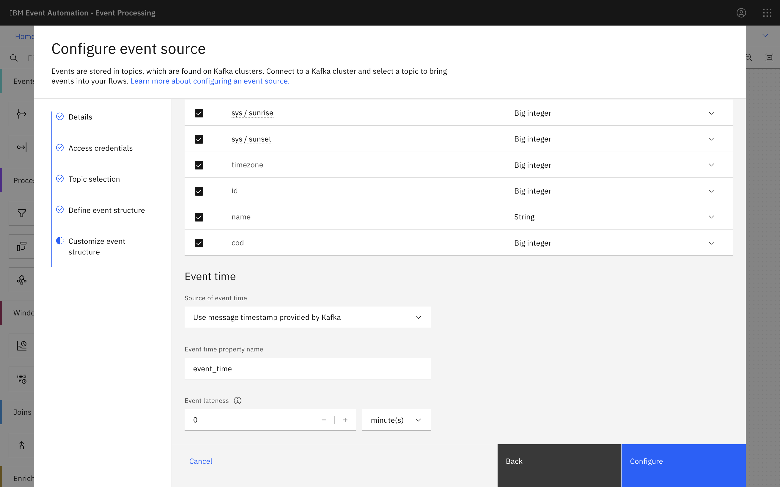
To see what this looks like as an event, you can see an example event that I captured. And to see an explanation of what all of this means, see the OpenWeather API documentation.
Bringing this topic into Event Processing looks like this:
Aggregating
The aggregate node in Event Processing makes it easy to calculate hourly summaries of the weather measurements.

There are lots of aggregate functions available to choose from. I picked a selection including AVG, MIN, MAX, and STDDEV_POP.

I repeated this for several of the values in the raw events.
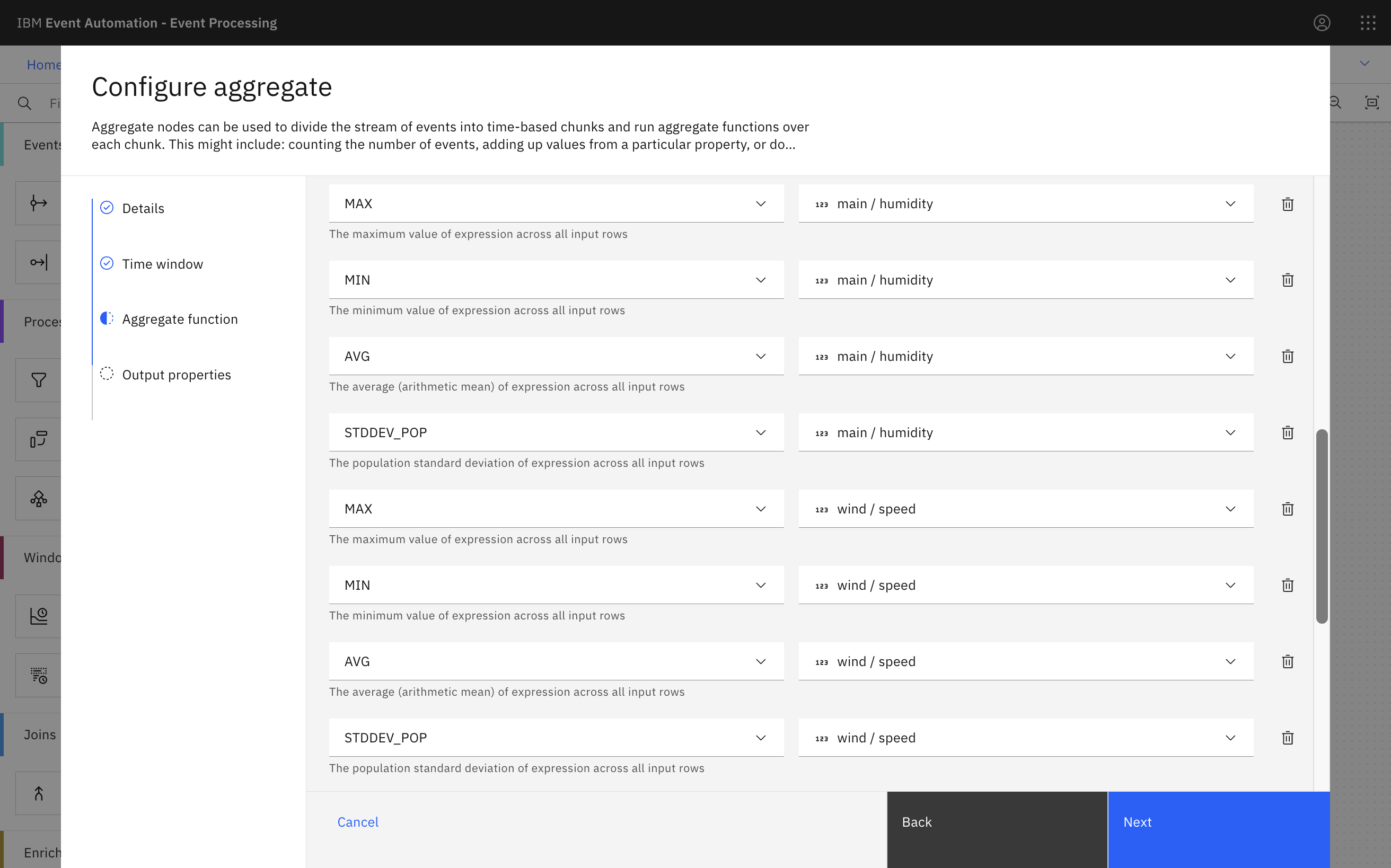

Giving the results friendly names makes it easier to use them in processing.


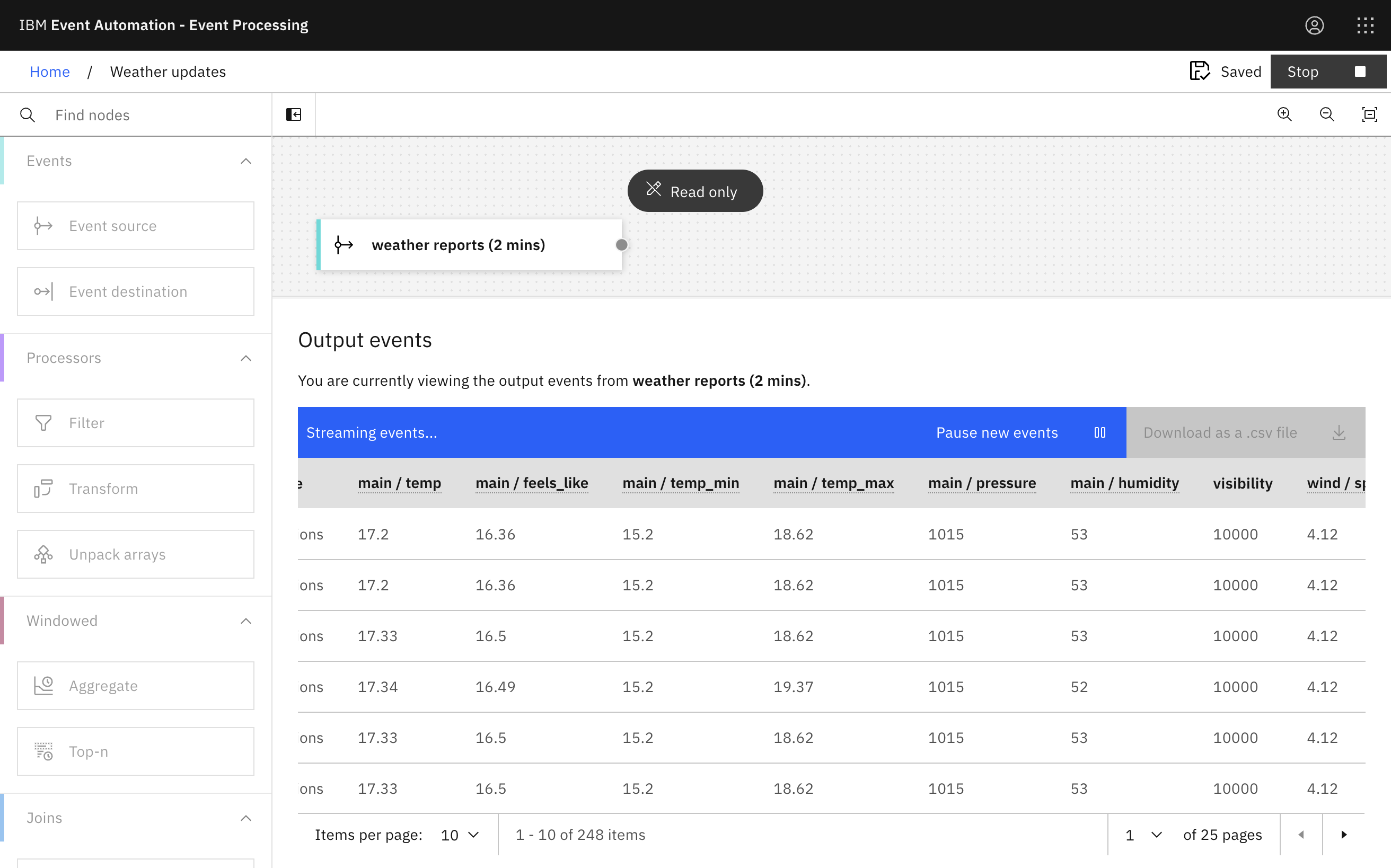
Running this looks like this:

watsonx
The first step is to generate a summarization prompt to use for the model. This can be done using the transform node in Event Processing.

The template I wrote for the prompt is below.
It looks complex, but there is a lot of repetition in there, as it just provides each of the aggregate values with enough context for it to be understood by the model.
CONCAT(
    'Measurements from a weather station in Compton, GB were taken ',
    'every two minutes between ',
        DATE_FORMAT(`start`, 'yyyy.MM.dd HH:mm:ss'), ' and ',
        DATE_FORMAT(`end`, 'yyyy.MM.dd HH:mm:ss'),
    '\n\n',
    'Temperature ranged between ',
        CAST(ROUND(`temperature min`, 1) AS STRING), ' and ',
        CAST(ROUND(`temperature max`, 1) AS STRING), ' degrees Celsius. ',
    'The average (mean) temperature was ',
        CAST(ROUND(`temperature average`, 1) AS STRING), ' degrees. ',
    'The population standard deviation of temperature measurements was ',
        CAST(ROUND(`temperature standard deviation population`, 3) AS STRING),
    '\n\n',
    'Pressure ranged between ',
        CAST(`pressure min` AS STRING), ' and ',
        CAST(`pressure max` AS STRING), ' millibars. ',
    'The average (mean) pressure was ',
        CAST(ROUND(`pressure average`, 0) AS STRING), ' millibars. ',
    'The population standard deviation of pressure measurements was ',
        CAST(ROUND(`pressure standard deviation population`, 3) AS STRING),
    '\n\n',
    'Humidity ranged between ',
        CAST(`humidity min` AS STRING), ' and ',
        CAST(`humidity max` AS STRING), ' percent. ',
    'The average (mean) humidity was ',
        CAST(`humidity average` AS STRING), ' percent. ',
    'The population standard deviation of humidity measurements was ',
        CAST(`humidity standard deviation population` AS STRING),
    '\n\n',
    'Wind speed ranged between ',
        CAST(ROUND(`wind speed min`, 1) AS STRING), ' and ',
        CAST(ROUND(`wind speed max`, 1) AS STRING), ' metres per second. ',
    'The average (mean) wind speed was ',
        CAST(ROUND(`wind speed average`, 1) AS STRING), ' metres per second. ',
    'The population standard deviation of wind speed measurements was ',
        CAST(ROUND(
            IF(`wind speed standard deviation population` > 0,
                    `wind speed standard deviation population`,
                    0),
            3) AS STRING),
    '\n\n',
    'Cloudiness measurements (as a percentage of sky covered) ranged between ',
        CAST(`cloudiness min` AS STRING), ' and ',
        CAST(`cloudiness max` AS STRING), ' percent. ',
    'The average (mean) cloudiness was ',
        CAST(`cloudiness average` AS STRING), ' percent. ',
    'The population standard deviation of cloudiness measurements was ',
        CAST(`cloudiness standard deviation population` AS STRING),
    '\n\n',
    'Generate a short, non-technical, easy to understand explanation of these ',
    'weather measurements for this 1 hour period. ',
    'Explain what the measurements indicate, such as by describing how it would ',
    'have felt to someone outside during this time.',
    '\n\n',
    'Use language that is suitable for a weather report in a newspaper, but ',
    'write in past tense as this is a historical report of previous weather.',
    '\n\n',
    'Avoid using technical or statistical jargon. ',
    'Do not include statistical terms such as population standard deviation in your summary.'
)
As with the stock activity demo, I didn’t spend any time refining this prompt either. If you would like to improve on this, you can use my example of the sort of prompt this creates to experiment with your favourite large language model. (If you come up with a new prompt that results in a more interesting summary, please let me know!)
This transform node can also remove all the properties that aren’t needed any further in the flow.

The API Enrichment node in Event Processing lets you enrich the content of events with data retrieved from external REST APIs. It’s useful when you want to process events in the context of reference data from a system of record.
For these demos, I’m using it to invoke a watsonx API.
I used the same simplified version of the watsonx API that I prepared for the stock prices demo.
As with the stock activity demo, I selected granite-13b-chat but I suspect there would be value in experimenting with the other models that are available to see if another model is better at this sort of task.

The API Enrichment node can also rename properties and remove properties that aren’t needed, to specify the final output of the flow.
Destination for results
The final step is to sink the output to a new topic.

As above, this could be used to trigger notifications containing these generated updates. Or sinking it to a database could be used to provide this content to a web app.

Tips for building flows like this
There is a cost associated with using generative AI APIs like watsonx, so it is worth creating flows with this in mind.
A couple of steps that I find useful for this are:
Using a mock API during development
A mock REST API that just returns a hard-coded response is a useful placeholder while you’re working on your Event Processing flow. I used App Connect for this, creating an API that returned “This is the response” with the same payload shapes as my real API.

This meant I could run my Event Processing flow many times while I was working on it, without worrying about making a large number of calls to the watsonx API.
Using a filter to limit the events during development
When working on flows that aggregate an hour’s worth of events, you need to run the flow with historical events to quickly see results from it. But if the source topic has many weeks worth of events on it, you don’t want to be instantly submitting thousands of API calls to watsonx every time you try out your flow.
I used an extra filter node during development, immediately after the event source. It only kept events with a recent timestamp, so that I would only get a single hourly aggregate.

This meant I could run my Event Processing flow many times while I was working on it, with each time only resulting in a single API call to watsonx.
Tags: eventautomation