I’m often asked this. The specific question varies, but it’s typically some variation of asking how quickly a single CPU of Flink processes events from a Kafka topic.
Why “per CPU”? Maybe because enterprise software is typically charged per CPU? Maybe because I tend to talk to people who run everything in Kubernetes, who think of running software in terms of requests / limits? Not sure, but the question tends to be framed from the perspective of asking how much processing they can expect to get from a CPU.
I try to avoid doing the engineer thing of answering “it depends“… but… it really does depend!

That is the motivation behind this post: to give me something I can point at as an illustration of the degree to which Flink’s performance varies (and a taste of the range of interrelated factors that influence it).
How different can it be?
I’ve talked before that my go-to example when demo’ing Flink SQL for now are Flink SQL flows that process click tracking events in a retail scenario. They are easy to explain, easy to understand, and let me show a variety of Flink SQL features.
Using that Kafka topic, and those sorts of flows as a basis, how fast do the Flink jobs I demo consume events (if I set the CPU limit to 1 for the job manager and task manager)?
I ran those flows a bunch of times, changing some configuration options along the way, to see what sort of range of speeds I could get as a result. When I plot each Flink job onto an x-axis based on the number of records it processed per second, I get:

Look at the range there.
At one end, one of the flows consumed approximately 1,340 events per second.
At the other end, another job consumed approximately 44,320 events per second.
TLDR – If you takeaway nothing else from this post, that’s the message. All of those flows were Flink running in the same place, consuming the same type of data, from the same Kafka cluster, using the same amount of CPU and memory.
The throughput varied massively depending on the type of processing the flow was doing, the type of data it was consuming, and how Flink was configured.
These results are specific to my environment, workload, and the configurations I tried. (And I took some questionable shortcuts that I describe below!) I’m sharing this as an interesting illustration of how variable Flink performance can be, and as an encouragement of the value of testing and benchmarking.
In other words, I guess I’m still saying it depends. 😉
Digging into the differences
If you hover over the points in the visualisation above, the tooltip gives an overview of what I did in that Flink job.
Seeing all of them in one group is helpful to get a feel for the distribution, but it doesn’t make it easy to see patterns. While I’ve got this data, it’s worth poking at it a little closer.
For example, let me pick out two of the Flink job runs. These two Flink jobs both:
- included an interval join (with a one-hour interval) between the click tracking topic and a second low-frequency topic
- included a session window (using a one-hour session gap)
- performed the same processing
- consumed the same events from the same source topics
The only thing I changed between these two runs was the configuration option I used for the state backend (where Flink held its state): either in memory using a hashmap, or in a persistent key-value store using RocksDB.
Putting these two Flink jobs side-by-side on a slope chart, I get:
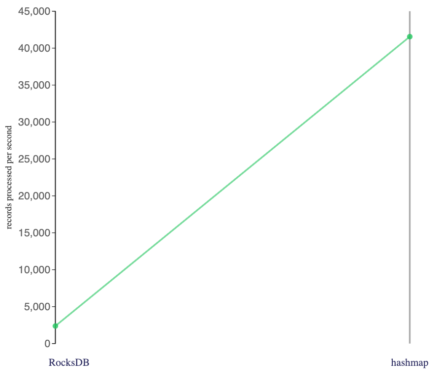
The job I ran using the hashmap state backend went a lot faster than the job I ran using the RocksDB state backend.
Impact of the state backend
What if I add all the other stateful Flink jobs I ran to that slope chart?
In other words, here are all the Flink jobs I ran that included an interval join, or a session window, or both.
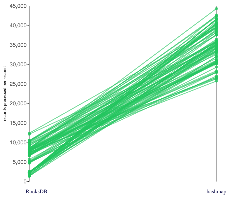
Some of these jobs consumed Avro events, some consumed JSON. Some consumed events that were compressed, some consumed uncompressed events. And so on. Each line is a different Flink job or configuration.
The slope chart connects Flink jobs that were implemented and configured identically, except for the state backend.
All of these jobs above were stateful in some way. Some consumed from only a single topic using a session window – others consumed from two topics correlating with an interval join, in addition to using a session window.
But what if I draw the slope chart with the stateless Flink jobs I ran?
For the purposes of this post, by “stateless” I mean Flink SQL that included no interval join and no windowed aggregates (rather than more general use of state in Flink or the Kafka consumers).
Here are Flink jobs I ran that did not make any use of state and used complex string functions (e.g. multiple uses of string parsing, regular expressions, etc.) on Avro format click-tracking events:
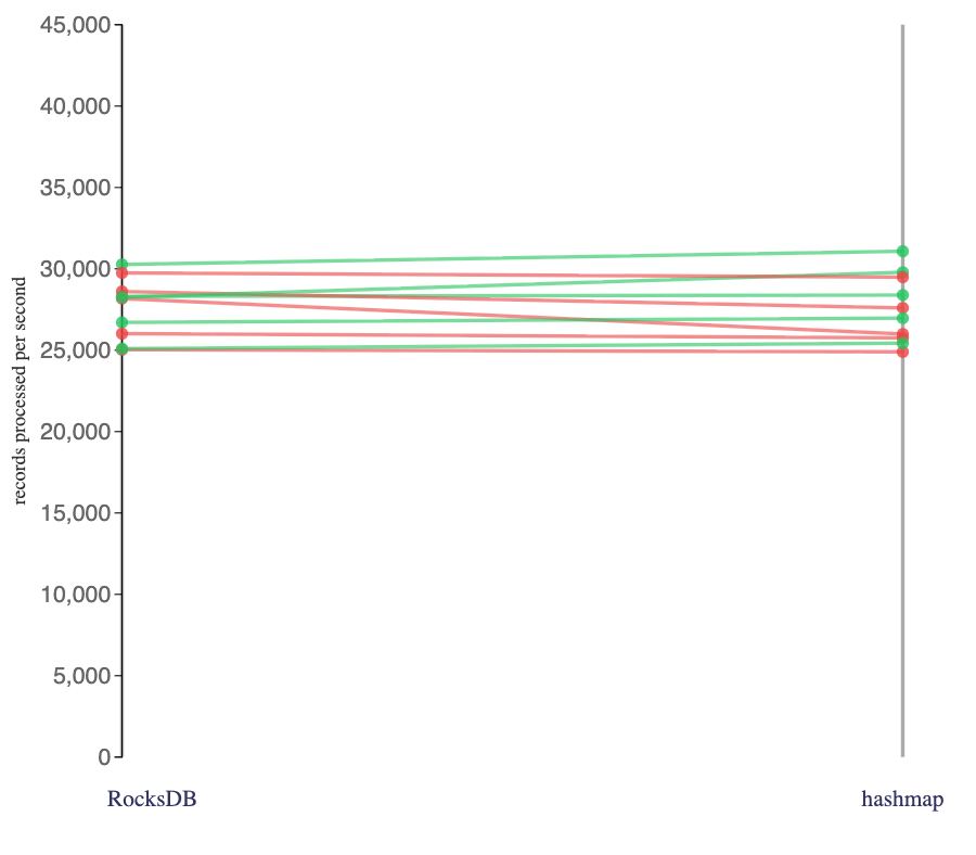
Green lines means the number of records processed per second increased. Red lines means the number of records processed per second decreased.
I’m not doing formal performance testing here. For one thing, I ran all of this on my development cluster, which is a shared environment. In the absence of an isolated environment, variation between runs is inevitable.
The choice of state backend made no significant difference in the speed of these Flink jobs I ran that didn’t use state.
So far, so obvious, right? When I ran Flink SQL jobs that made heavy use of state, they ran faster using a memory-based state store than they did using a disk-based state store. When I ran Flink SQL jobs that didn’t use state, it didn’t make much difference either way. I would’ve predicted that, but it’s reassuring to see it confirmed.
It wasn’t all so obvious. When I add all of the stateless Flink jobs I ran onto the chart:
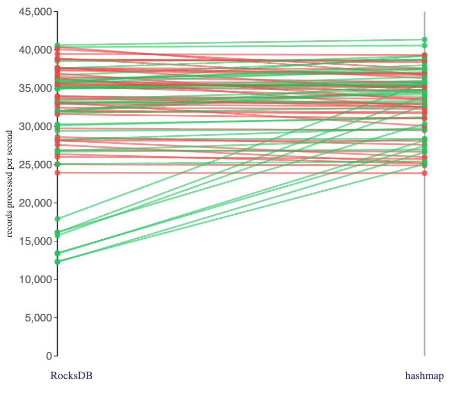
In other words, this shows not just the ones using Avro source topics, and not just the ones that included complex string functions, etc.).
These results are a little harder to explain. I think this still shows that the state backend had a mostly minimal impact, but there were a small collection of jobs that seemed to go faster which I haven’t properly understood.
All the stateful Flink jobs I ran went faster when I used a hashmap backend. Does this mean I would always use hashmap for stateful jobs?
Not necessarily. For one thing, some Flink jobs hold so much state that it’s just not feasible to give them enough memory. For some jobs, the amount of state varies so much it’s not efficient to give them enough memory to guarantee it will have enough to always hold the entire state.
There are other considerations, too – some of which I’ll get to below.
Impact of the processing complexity
Looking at the stateless jobs a little closer, I ran a few different types of stateless Flink SQL jobs on my click tracking events. I created Flink jobs that did:
- no processing – only deserialized source events and sinked them
- simple – only performed numeric operations on source events
- complex – performed complex string functions, including multiple uses of string parsing, regular expressions, etc.
Looking at the impact of the type of processing on these stateless jobs:
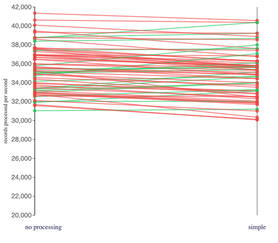
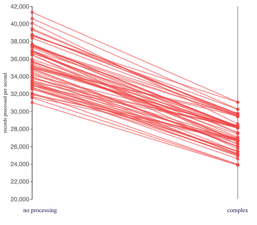
The impact of the more CPU-intensive string parsing functions in the “complex” jobs had a noticeably larger impact on the speed of the jobs that I ran.
Any processing reduced the number of events that Flink processes per second compared with not doing any work at all.
Numerical functions were unsurprisingly efficient and had only a minimal impact on the job’s speed.
When I included string parsing and regular expression functions in my stateless jobs, I reduced the number of events my Flink jobs processed per second by nearly 25%.
Impact of the format of source events
I created separate versions of the source topics that the Flink jobs could consume from: JSON and Avro.
Comparing the performance of Flink jobs that (were otherwise identical other than whether they) consumed from the JSON or Avro topic:
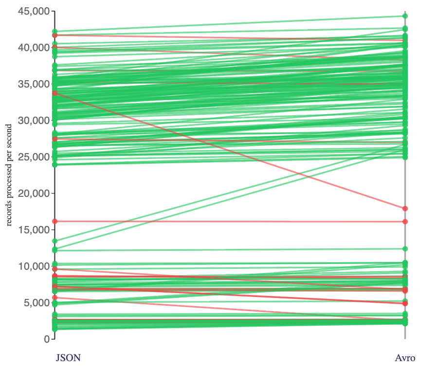
For this setup, my Flink jobs that consumed Avro events almost always processed events more quickly than the Flink jobs that consumed JSON events. But the benefit that Avro brought was not consistent across all types of jobs that I ran.
For example, looking at stateful jobs (jobs that included an interval join and/or session window aggregates) that consumed from topics where the Kafka producers had not used compression:
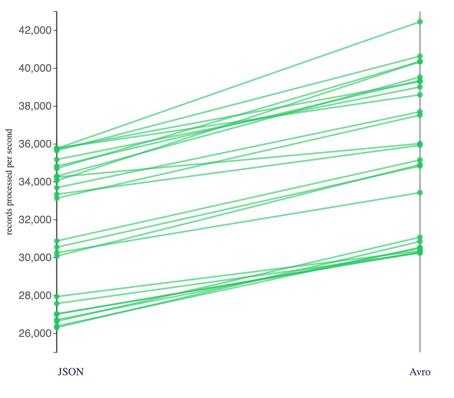
In other words, in these jobs, the Flink jobs in the left category were consuming a large amount of whitespace in multi-line, pretty-printed JSON events, with a large number of JSON keys repeated multiple times in the consumed data. This was JSON at its worst, and showed the most significant benefit from using Avro.
Compare that with these stateful Flink jobs consuming from topics where Kafka producers had used compression and large batch sizes:
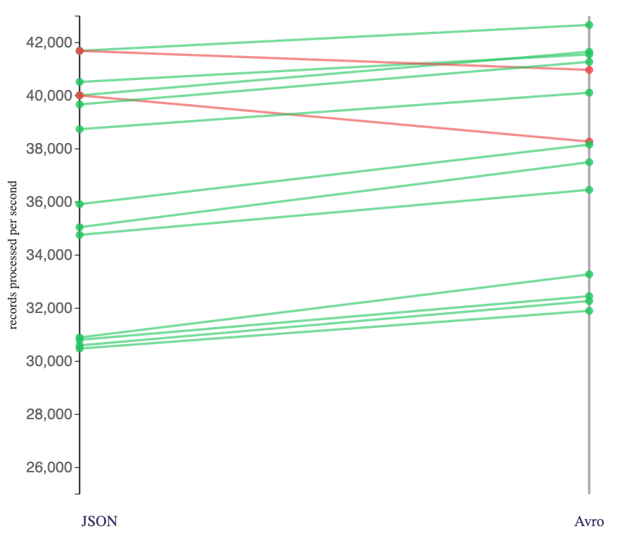
Avro topics still showed a performance benefit for most jobs, but this was more modest. When Kafka producers had used compression and large batch sizes, this had mitigated some of the costs of JSON.
Looking at the impact of source format on stateless Flink jobs that did no processing (i.e. jobs that only deserialized source events and sinked them):
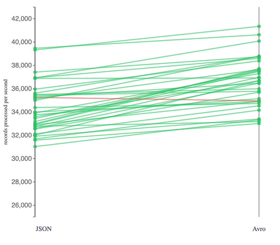
Again, the Flink jobs almost always processed events from Avro topics at a faster rate than JSON. The benefit was also more modest.
Deserializing Avro events typically requires less CPU than deserializing JSON events. These Flink jobs would not have been CPU constrained, so the benefit they gained from CPU cycles freed up by deserialization were perhaps reduced.
This is a difficult aspect to try and discuss in isolation.
In theory, processing Avro events rather than JSON brings network transfer benefits (my JSON events were larger than their Avro equivalents, so Flink’s Kafka consumer could consume more Avro events more quickly than JSON). In a network-constrained environment, this could be hugely important.
But in a low-latency network environment, or even if the Flink job processing was so complex that the source was backpressured, then this benefit is reduced – it potentially just increases the time the source spends backpressured.
In theory, processing Avro events rather than JSON brings CPU benefits (deserializing JSON requires more CPU than Avro).
But if the Flink job is not CPU constrained, then this benefit is reduced – it potentially just increases time that the CPU is spent idle.
Using Avro instead of JSON seemed to consistently improve performance. But the degree to which it improved performance was diminished in some runs impacted by other factors.
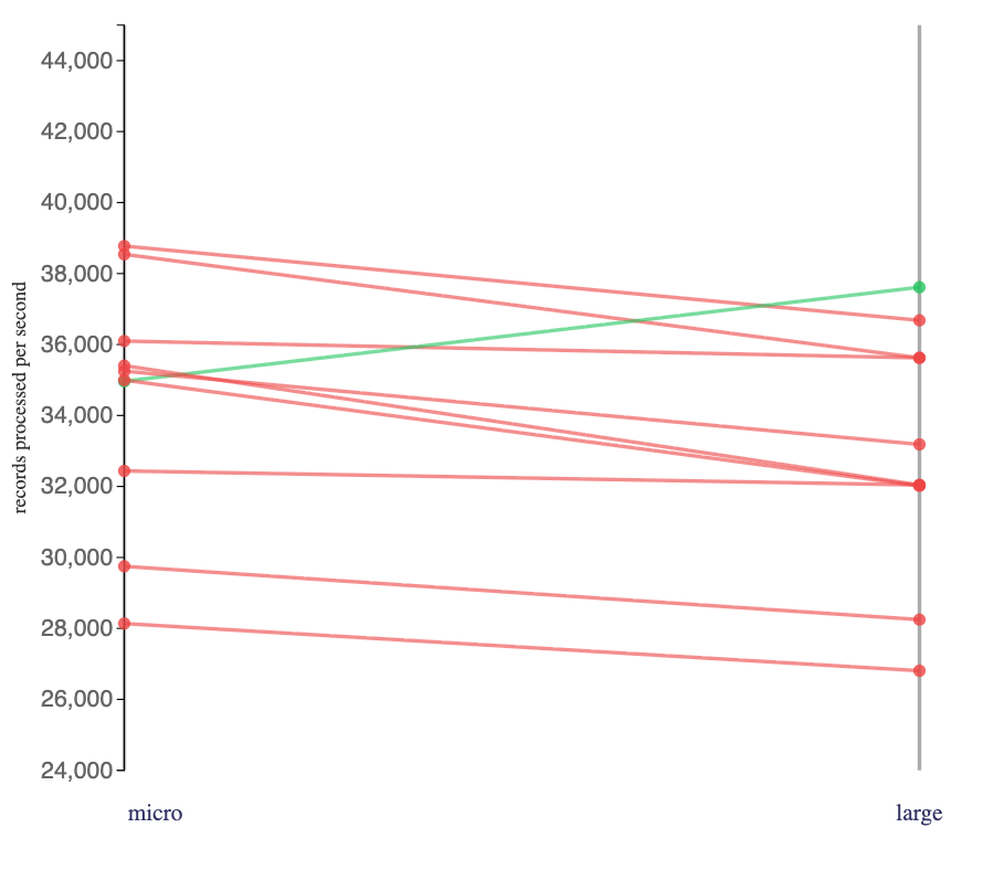
Impact of producer batching
Kafka brokers cannot send partial batches from a topic, so the size of batches that a producer sends to a topic will influence the amount of data that Flink job will receive when it fetches from its Kafka source.
To see the impact of producer batching, I set up versions of the click tracking topics where producers used:
- “micro” – tiny, single-message batches
batch.size: 0 - “large” – larger-than-default batches
batch.size: 409600, linger.ms: 10000
Flink jobs consuming from the “micro” topics will have received a large number of single-message batches in each poll.
Flink jobs consuming from the “large” topics will have received a couple of multiple-message batches in each poll.
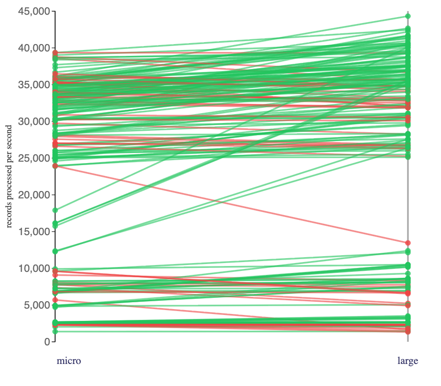
The impact of this on the rate that the Flink jobs I ran was mixed. Two thirds of the jobs faster with the larger batches, one third went slower.
There were Flink jobs where it always went faster, such as stateful jobs using a hashmap state backend to consume compressed batches:
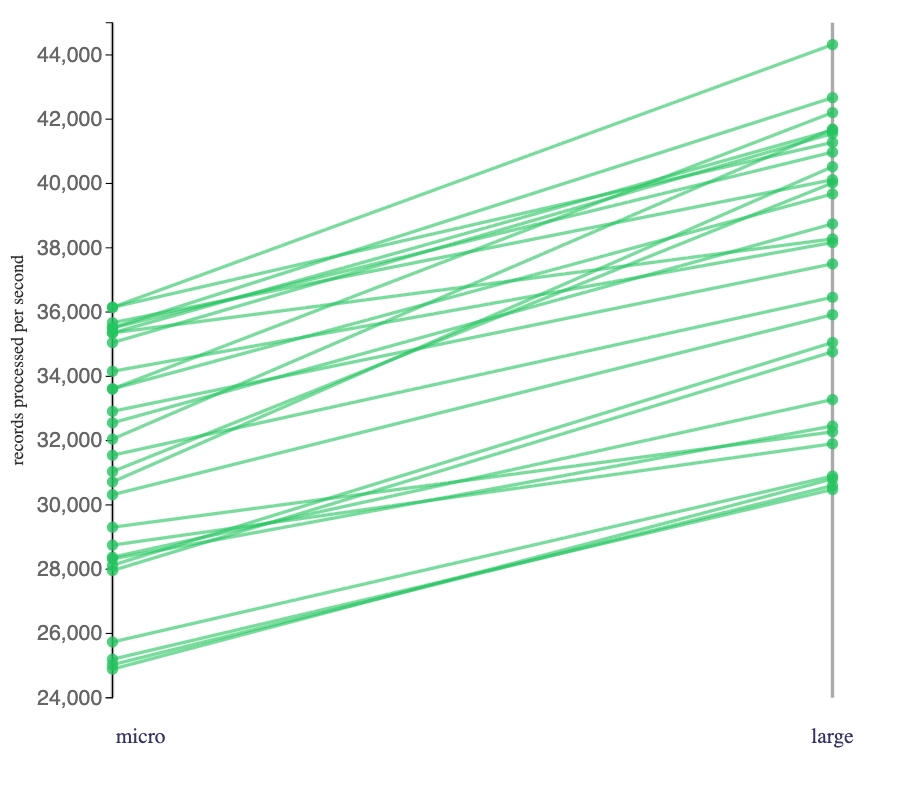
There were Flink jobs where it didn’t help, such as stateless jobs that consumed uncompressed batches:
Impact of producer compression
If producers compress the batches they send to Kafka, Kafka consumers need to decompress the batches before deserializing the events. This could reduce the network traffic the Flink job needs to wait for when receiving events from its source, however it also introduces a CPU overhead for Flink to decompress each batch it receives.
To see the impact of producer compression, I set up versions of the click tracking topics where producers used:
- “uncompressed” – no compression
compression.type: none - “compressed” – compression using
compression.type: snappy
Looking at the impact of compression on the Flink jobs that consumed from the “micro”-batch topics:
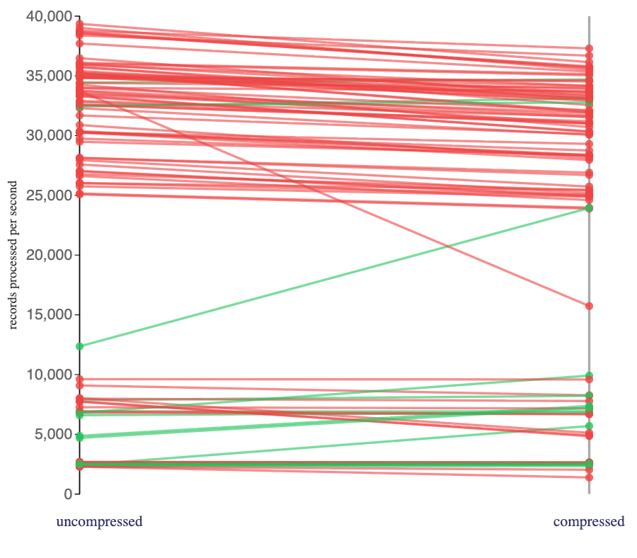
The compressed topics slowed down almost all of these Flink jobs.
Compression is applied at a per-batch level. Its effectiveness is dependent on the presence of repeated data in the batch.
Producers using single-message batches with compression is inefficient. It doesn’t reduce the data size (it could have even increased the data size).
It still introduced a CPU overhead for consumers needing to decompress data before deserializing, and this can be seen in the impact that it had on how many click tracking events my Flink jobs processed per second from the “compressed” topics.
Looking at the impact of compression on Flink jobs that consumed from the “large”-batch topics when using a hashmap state backend:
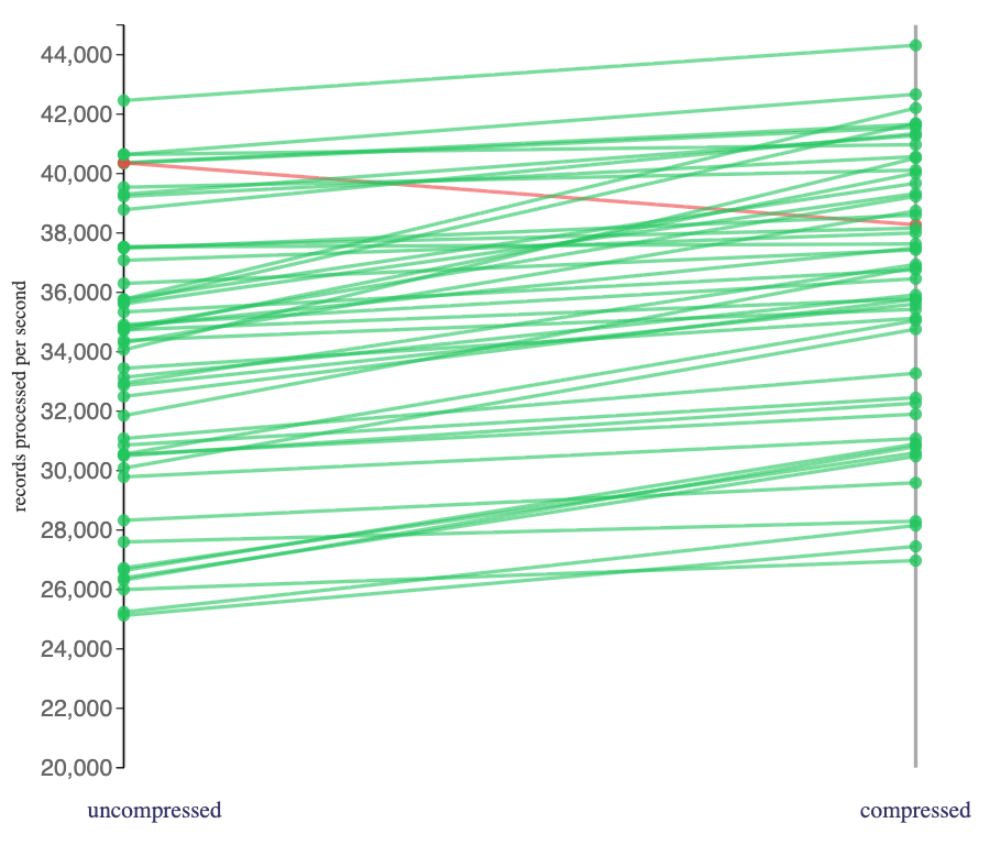
Large batches compress very well, so any additional CPU overhead of decompressing the batches that Flink incurred appeared to be outweighed in these jobs by the benefits of the more efficient network I/O.
Surprisingly, I didn’t see that consistent benefit from the impact of compression on Flink jobs that consumed from the “large”-batch topics when using a RocksDB state backend:
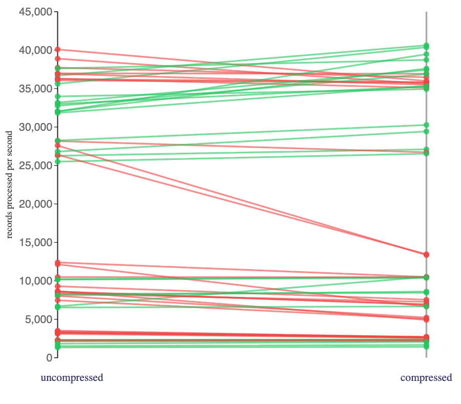
Perhaps some of these Flink jobs were sufficiently CPU bottlenecked that the additional overhead of decompression became a more significant cost. There may be other explanations. Because I only collected a single metric (the number of records in the Kafka source) for these jobs, I can’t get any deeper understanding of the behaviour.
Okay, Kafka producers configured to use compression and batch.size of 0 is contrived, and not something you are likely to come across.
I’m using this to illustrate that the number of records a Flink job can process per second is influenced by the configuration choices made by the Kafka producer that created the records your Flink job is processing (even when you don’t change any configuration of your Flink job).
What I’m showing here is an extreme example of this.
Impact of using interval joins
Some of the Flink jobs I ran included an interval join with a second, low-throughput topic. For those jobs, I was correlating the high-throughput click stream topic with a second topic of new customer registrations.
Comparing the Flink jobs I ran that:
- “no join” – did not include an interval join
- “join” – included an interval join
(but were otherwise consuming the same events from the same topics and doing the same processing, configured in the same way), I get:
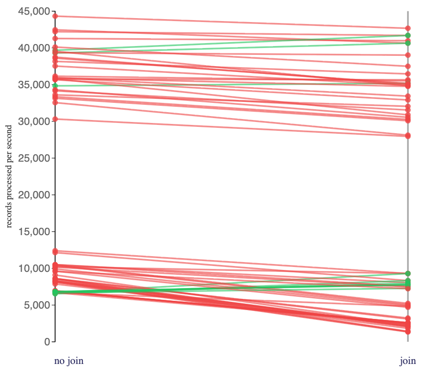
I saw a small, but mostly repeated, reduction in the rate that Flink could consume the click tracking events when I included an interval join.
The top group are all Flink jobs using a hashmap state backend.
The bottom group are all Flink jobs with a RocksDB state backend.
It’s worth noting that the impact here won’t solely have come from the JOIN itself – the Flink jobs I ran that included an interval join needed a second Kafka source for the second topic. In addition to the additional Kafka consumer, the Flink job had a another topic to deserialize events for. While I intentionally chose a very low-throughput second topic to minimise this, the impact won’t have been nothing.
I also tried two different options for the interval join duration, to see the impact of interval duration on the number of records processed per second.
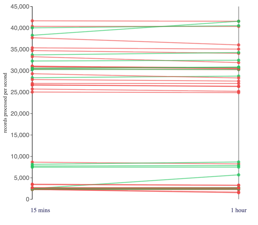
I tried two variations: using a 15 minute interval, and using a 1 hour interval. I expect that the Flink job runs in the right category will have stored roughly 4 times as much state as the job runs on the left.
This didn’t seem to make much difference.
Across the variety of Flink jobs that I ran, I saw jobs using an interval join processed click tracking events slower than jobs that didn’t, but this reduction was small.
The duration of the interval join didn’t appear to make a significant difference. This is perhaps because on my topics, the matches to be found mostly occured within the smaller 15 minute interval anyway, and would not have significantly changed the output. As a result, the impact primarily comes from consuming and deserializing events from a second topic, and having to do a lookup on every click tracking event – all of which was work that was needed whatever the size of the state that it is doing the lookup in.
Impact of using session window aggregates
Some of the Flink jobs I ran aggregated click tracking events within a session window, computing aggregates for click events by the same user that were part of the same session.
- “no window” – did not include any windows
- “window” – used a session window to aggregate click events with the same sessionid
Comparing the impact of including session window aggregates on Flink jobs that I ran that used a hashmap state backend:
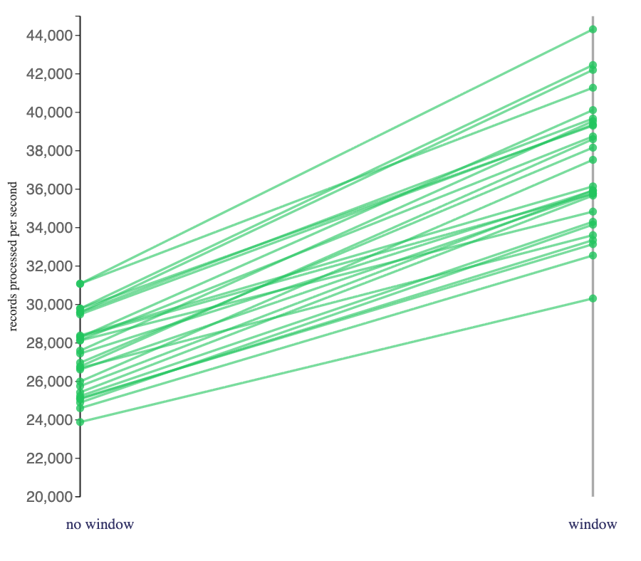
My Flink jobs using a session window consistently consumed click tracking events at a faster rate than the equivalent jobs without a session window (when I used a hashmap state backend).
The Flink jobs without a session window were outputting something for every click tracking event input. The Flink jobs using a session window only produced output when each session window closed.
For example, if Bob spends ten minutes clicking around the retail site, generating thirty separate click events, the Flink jobs without a session window would output 30 events about Bob, the Flink jobs with a session window would output 1 event about Bob.
Perhaps the reduced amount of output needing to be serialized freed up resource to allow the Flink jobs to process the click tracking events more quickly, even after the cost of maintaining the session state and computing the aggregates.
Comparing the impact of including session window aggregates on Flink jobs that I ran that used a RocksDB state backend:
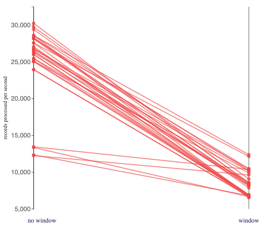
My Flink jobs using a session window consistently consumed click tracking events at a slower rate than the equivalent jobs without a session window.
These jobs should have benefited from the same reduction in output that the hashmap jobs did. I assume that this was outweighed by the increased cost in updating a disk-based state store in response to every click tracking event, and having to retrieve the state from a disk-based state store when computing aggregates.
I also tried two different options for the session window gap, to see the impact of session window size on the number of records processed per second.
Looking first at the impact on Flink jobs using a hashmap state backend:
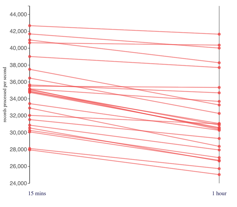
I tried two variations: using a 15 minute session window gap, and using a 1 hour session window gap.
The longer session window caused a relatively small, but consistent, reduction in the rate that click tracking events were processed.
The jobs will have produced mostly the same output either way, the difference is that the jobs on the right will have waited for a longer time for the session gap to be exceeded before computing and outputting the aggregates.
Looking at the impact of session window size on the Flink jobs that used a RocksDB state backend:
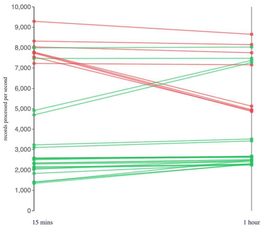
The impact here was more mixed.
Using a session window significantly reduced the amount of output that my Flink jobs produced for this scenario.
This is perhaps why I saw an increase in number of records they processed per second when the cost of state this required was cheap (using a hashmap state backend) but a decrease in the number of records processed per second where the cost of using state was expensive (using a RocksDB state backend).
Impact of checkpointing
Looking still at the results for the most stateful Flink jobs that I ran (the jobs that included both an interval join and a session window), I ran them with:
- “no checkpoints” – checkpointing was disabled
- “checkpoints” – checkpoints were created every 30 seconds
The impact of enabling checkpoints on stateful jobs that used a hashmap state backend.
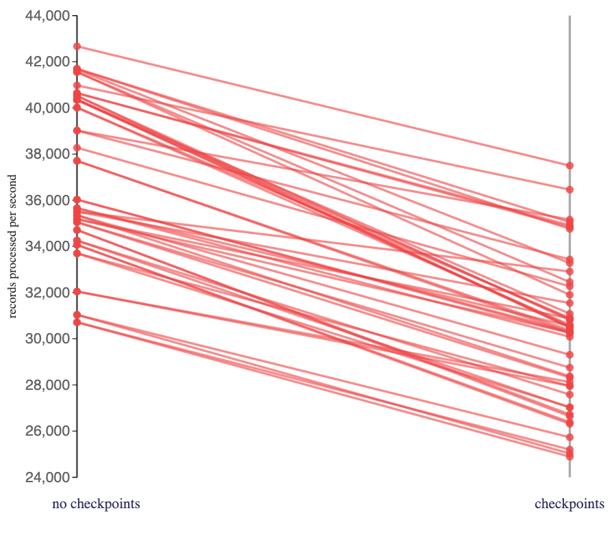
As I expected, there was an impact in requesting that Flink periodically save its state to files. Checkpoints bring resiliency across crashes and restarts, so I consider them worth the cost, but it was interesting to see the degree of impact it had on these particular click-track processing jobs.
Looking at the impact of enabling checkpoints on stateful jobs that used a RocksDB state backend.
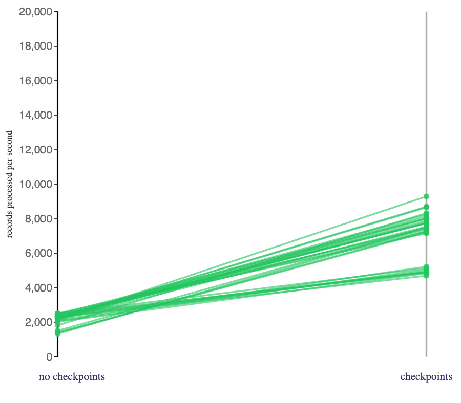
These jobs went significantly faster when I enabled checkpoints. I wasn’t expecting that.
When I changed the checkpoint interval, from the 30 seconds shown above, to 15 minutes (still showing stateful jobs that used a RocksDB state backend):
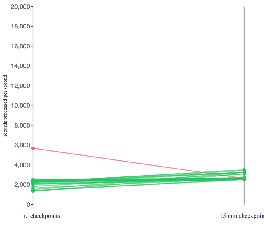
There was still a speed benefit from creating checkpoints (which still surprised me), but checkpointing less frequently reduced the benefit. This was the opposite of what I expected – I’d incorrectly assumed that (if you don’t mind the increased recovery time) checkpointing less frequently would tend to reduce the impact of doing checkpointing.
This sent me down a fascinating rabbit-hole… “Managing Large State in Apache Flink: An Intro to Incremental Checkpointing” talks about incremental checkpointing triggering “a flush in RocksDB, forcing all memtables into sstables on disk, and hard-linked in a local temporary directory”.
And the RocksDB tuning guide has a whole section on the impact of flushes and compactions on RocksDB performance. There is a whole world of tuning info for RocksDB in Flink that I haven’t properly explored, so I can’t claim deep expertise here.
Ultimately, for the small number of Flink job runs I did as part of this, the performance of the more stateful jobs benefited from checkpointing. Perhaps this was because the incremental checkpointing was triggering RocksDB compaction and memtable flushes, which prevented the LSM tree from fragmenting or bloating as much as it did when I ran the Flink job with checkpointing disabled. But with only a single metric (the number of records per second in the Kafka source), there’s no way to know without a proper analysis.
This may well have been an edge case that applies for my specific types of flows or the click tracking events I was processing. I don’t assume that this is a generally applicable tuning recommendation, but I was still pleased to learn some new Flink stuff from doing this!
Summary
What about…?
There are so many aspects I didn’t explore.
Perhaps most importantly, I didn’t explore the impact of parallelism. All jobs I ran had a max parallelism of 1 on a single CPU core, consuming from single partition topics. This constraint must have been influential. For the Flink jobs that appear to have been bottlenecked on I/O (e.g. stateful jobs using a RocksDB state backend) there will have been time where the CPU was blocking on disk access. Increasing the parallelism would allow this idle time to be used on computations for other sub-tasks. It would have been interesting to see the impact this would have on throughput, even if I didn’t increase the CPU limit available to the task manager pod. This may well have outweighed the patterns I did observe.
There are other aspects I could’ve tried too, but even with the few factors I did try the number of permutations got out of hand!
What I did see
Ultimately, this was never meant to be exhaustive. I picked a few aspects that would be simple to alter, and that I suspected would have an easily noticeable impact. I did see some patterns in the performance of the Flink jobs that I ran:
- my stateful jobs ran faster when I used a hashmap state backend than when I used RocksDB (for stateless jobs, it made minimal difference)
- my stateless jobs ran slower as I used more complex functions
- my jobs consuming Avro data from topics ran faster than jobs consuming JSON data – but the amount of impact this had varied
- my jobs consuming from topics that had events in large, compressed batches went faster when using a hashmap state backend
- my jobs that included interval joins ran a bit slower than similar jobs without a join (the interval duration didn’t make much difference)
- my jobs that computed aggregates over a session window were slower (than similar jobs that didn’t use a session window) when using a RocksDB state backend, but faster than similar non-window jobs using a hashmap
- enabling checkpointing slowed down my jobs that used a hashmap state backend but sped up the jobs using a RocksDB state backend
All of this resulted in a wide spread in terms of how quickly my Flink jobs processed the same type of data.
What this means
But to be clear, this isn’t a benchmark. These results are specific to my jobs processing events from my topics. Don’t mistake this for a generic performance report.
At any rate, I’m not claiming that the ~45,000 events per second I saw in my fastest jobs I ran is particularly high or impressive. As I noted above, I didn’t run any of this on isolated hardware – it was all run on a low-spec virtualised development cluster, on a platform that I share with many other developers.
To avoid needing to alter memory limits between different jobs, I gave every job the same ridiculously large amount of memory. That probably masked some bottlenecks, and maybe even introduced other problems. This was a quick-and-dirty demonstration in a shared noisy environment, that’s all.
Please don’t misunderstand my intention here when I point out patterns I think are interesting in the data I happened to see in these particular jobs. I’m absolutely not claiming any of these as definitive rules or that they would apply to other types of Flink jobs processing other types of events or data.
More importantly, please don’t misinterpret anything here as tuning recommendations for your Flink job with your data. I’m not saying that setting option X or pulling lever Y will always make a Flink job run faster. I’m trying to say almost the opposite of that.
I’m saying that understanding how many Kafka events your Flink job will process per second will depend on an understanding of:
- the types of processing you include in your SQL
- how you tune and configure Flink
- a whole bunch of things you probably can’t control from Flink – such as the format of the events you’re processing, whether the events are compressed, how they are batched, and much more besides
Things that might reduce CPU usage in one area might be hugely beneficial for some jobs. For jobs that aren’t CPU bottlenecked in that area, it might have negligible impact.
As I described in my post on how I deploy Flink jobs in Kubernetes, part of deploying your job is to look at the metrics from your job running in your environment, and to use that to inform how you configure it.
If you really want to know the answer to “How many Kafka events will Flink process per second?“, there is no substitute for benchmarking and testing in a representative environment using a representative workload.
Flink is highly tunable, but the configuration options available to us are context sensitive. An understanding of your event data and your processing characteristics are essential to identify sensible configuration – in a way that blanket “turn on option X” rules won’t cover.
How I did this
My starting point was the sorts of Flink SQL flows I typically create in demos using click-tracking events. I created a few variations to give me jobs with/without interval joins, session windows, different types of stateless processing, etc. I ended up with seven basic types of Flink SQL flow.
I deployed these flows to the same Kubernetes cluster where my Kafka cluster was, using the Flink Kubernetes Operator and the approach I talked through last month.
All Flink jobs consumed the same click-tracking event data from single-partition topics on the same Kafka cluster, and all Flink jobs were run with a parallelism of 1.
All Flink jobs consumed from the earliest offset on the source topic, and ran until they had consumed three days (72 hours) of events. The topics had over 84 hours of events, so the Flink jobs were never allowed to catch up with the latest offset – they were consuming historical retained events as fast as they could. (The first 5 minutes of each Flink job activity was treated as startup and warmup time, and ignored for all of this.)
All Flink jobs were run individually – no other jobs were running at the same time.
All Flink jobs were run on the same k8s worker node, a worker node which didn’t host any of the Kafka brokers – to try and keep network latency between Flink and Kafka roughly consistent.
All Flink jobs were run on a task manager with CPU limited to a single CPU core, and a very high amount of memory available (20gb).
All Flink jobs used the same version of Flink (2.2).
When checkpointing was used (see below), incremental checkpointing was always enabled. When RocksDB was used (see below), it always used local disk storage.
I used numRecordsIn metrics from Flink for the click tracking Kafka source, averaged over the duration of the job, as a simplified representative proxy for how fast the Flink job was going. (For jobs that were also consuming a second topic to include an interval join, I ignored the metrics for this second Kafka source).
How I used Generative AI for this post
Orchestrating running the Flink jobs
I used an AI IDE to write the script that automated:
- generating a configmap with a set of configuration options to test
- starting the Flink job (by applying k8s custom resources for the FlinkDeployment and supporting configmaps and PVCs)
- polling the Flink REST API to:
- collect and average the metrics
- monitor the watermark for the click tracking event source to identify when the job had reached the target timestamp
- deleting and cleaning up the Flink job (by deleting the FlinkDeployment and supporting other custom resources)
- writing the results to a CSV file
- repeating this for the different permutations of configuration options to be tested
This meant I could leave this running in the background for a few weeks and forget about it, especially useful as I went on holiday!
Creating the visualisations
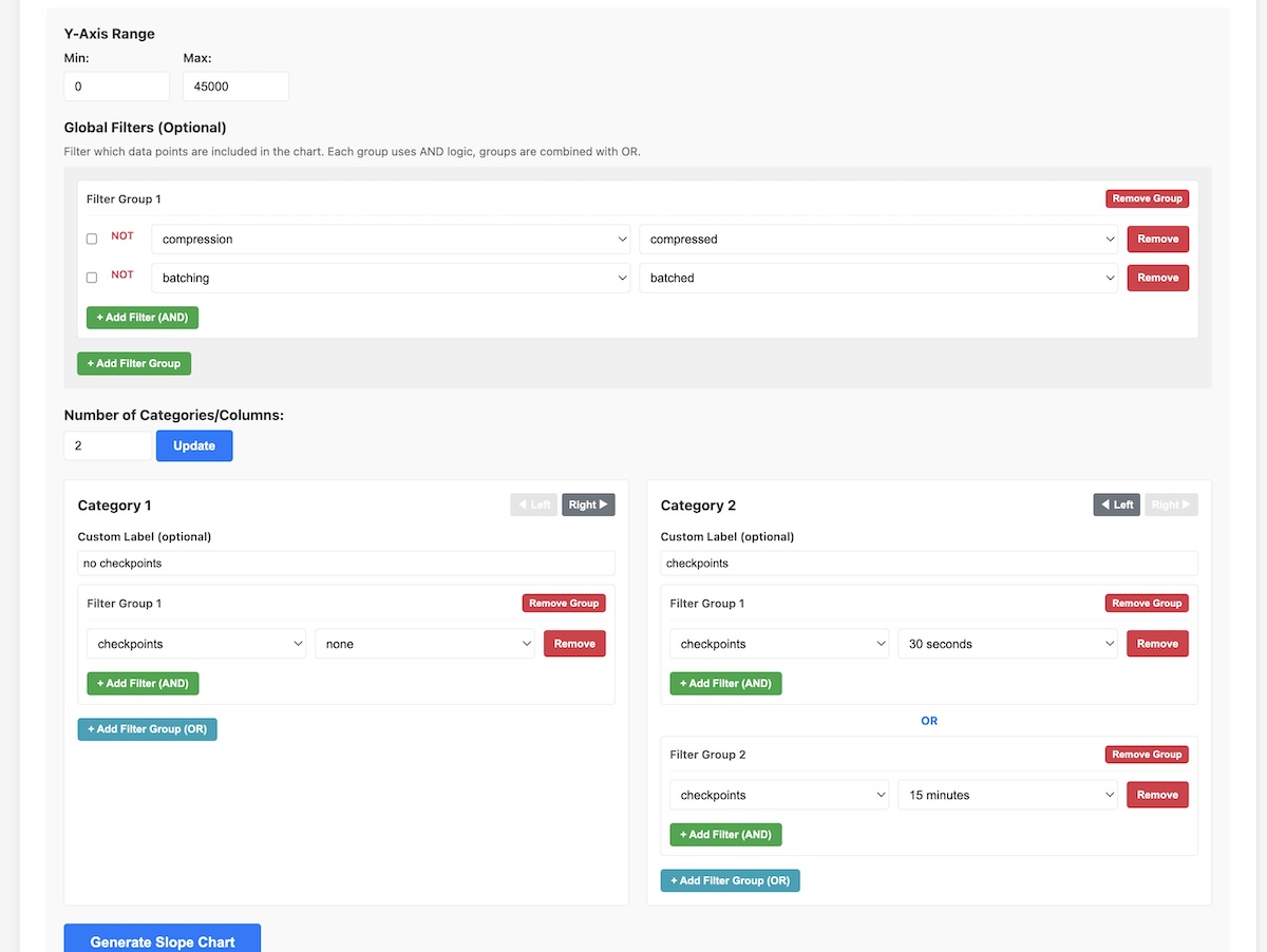
I also used an AI IDE to vibe-code a tool to generate slope charts – charts that I used to explore the data and then to illustrate this post.
The chart generator is a single-page HTML+JavaScript tool, that I’m the only user of, so I didn’t pay very much attention to the implementation other than to check it generates accurate charts.
Why AI?
I don’t think either of these are things that I couldn’t have done myself. But, it was quicker to let AI do them. GenAI meant that the jump from my idle thought of “I wonder what difference it’d make if I ran this Flink SQL job a bunch of times with different configs” to actually doing it was so small that this was an easy thing to kick off before heading home one Friday afternoon.
Tags: apacheflink, flink
Any chance you could fix the broken links? (Or get AI to do it!)
What broken links are you noticing?